Towards Fused Kernels for Gated MLP
The decoder block of a Transformer is the basic unit of all modern LLMs. Most of the compute used for it is spent on self-attention and the MLP, with self-attention in special being problematic on long sequences due to its quadratic compute and memory requirements. It is not surprising therefore that there's been a lot of progress towards increasing the performance of self-attention, such as FlashAttention [1], or algorithms and models that approximate full attention, like Window Attention [2], or State-Space Models [3, 4, 5]. While efficient kernels for MLPs do exist, from what we could find they seem to be either tailored to very specific setups, or only partially solve some of the issues of MLPs, such as fusing the gating operation.
We spent the last few weeks working on a kernel that computes the up-scaling and gating part of the MLP in a single (fused) call. In this blog post, we will explain our approach and dive into some low-level details of our implementation. While having some familiarity with GPU kernels will make reading this blog easier, we include some introductory sections that give a high-level overview of relevant concepts. The full implementation can be found at our GitHub repo.
Gated MLPs
Gated MLPs, introduced in [6], changed the activation used in the traditional MLP block from an element-wise nonlinearity to a gated linear unit (GLU). As seen in the below image, this adds more computation and memory usage, as it requires an extra up-scaling of the input.

The thin rectangles are activation functions.
This requires projecting the input tokens into a much larger dimension. For example, for Llama 405B the inputs are projected from to , where is the sequence length. This in turn means that when training with sequences with less than context length, the MLP will dominate self-attention in terms of FLOPs, because the quadratic cost in terms of context length is actually lower. In general, this holds for most sizes of LLMs, as even smaller models in the 8B class usually upscale to the 14k-20k range, which exceeds most context sizes used for pretraining. When paired with efficient attention kernels, this can also lead to the MLP utilising most activation memory during training.
For inference, the discussion is more nuanced. Inference engines tend to prioritize, among other things, storing as little memory as possible for activations to make room for larger models and KV caches. We will have a section towards the end of the post where we will discuss in more detail how exactly our kernel might fit in a modern inference engine, but briefly speaking, we expect the impact of our kernel to be modest in terms of memory, but still useful for further improving the throughput of model deployments.
GPU kernels
"Kernels" is the name given in GPU programming to functions that are executed in parallel on a GPU. More formally, "in parallel" refers to the Single Instruction Multiple Threads (SIMT) model, in which groups of threads (called warps for Nvidia chips) execute the same instruction in parallel, while operating on separate slices of data.
One classic example is to think of a function that grayscales an image. We can write a kernel that computes the color for a single pixel, and then run it on the GPU to transform the entire image in parallel. A kernel will have an associated Cooperative Thread Array (CTA), also called threadblock, which generally consists of multiple warps. Each warp will handle a patch of the original image. Since all the threads in a warp run in parallel, even if one single thread isn't particularly fast, we can still obtain high throughput from the parallel nature of execution. More so, all warps are also launched in parallel, although the degree to which they can execute in parallel is a much more nuanced discussion than in the case of threads in a warp 1 (suffice to say there is still a very large amount of parallelism).
While this explanation glosses over a lot of important details, we believe it is enough to follow the high-level overview of our kernel.
Kernel fusion
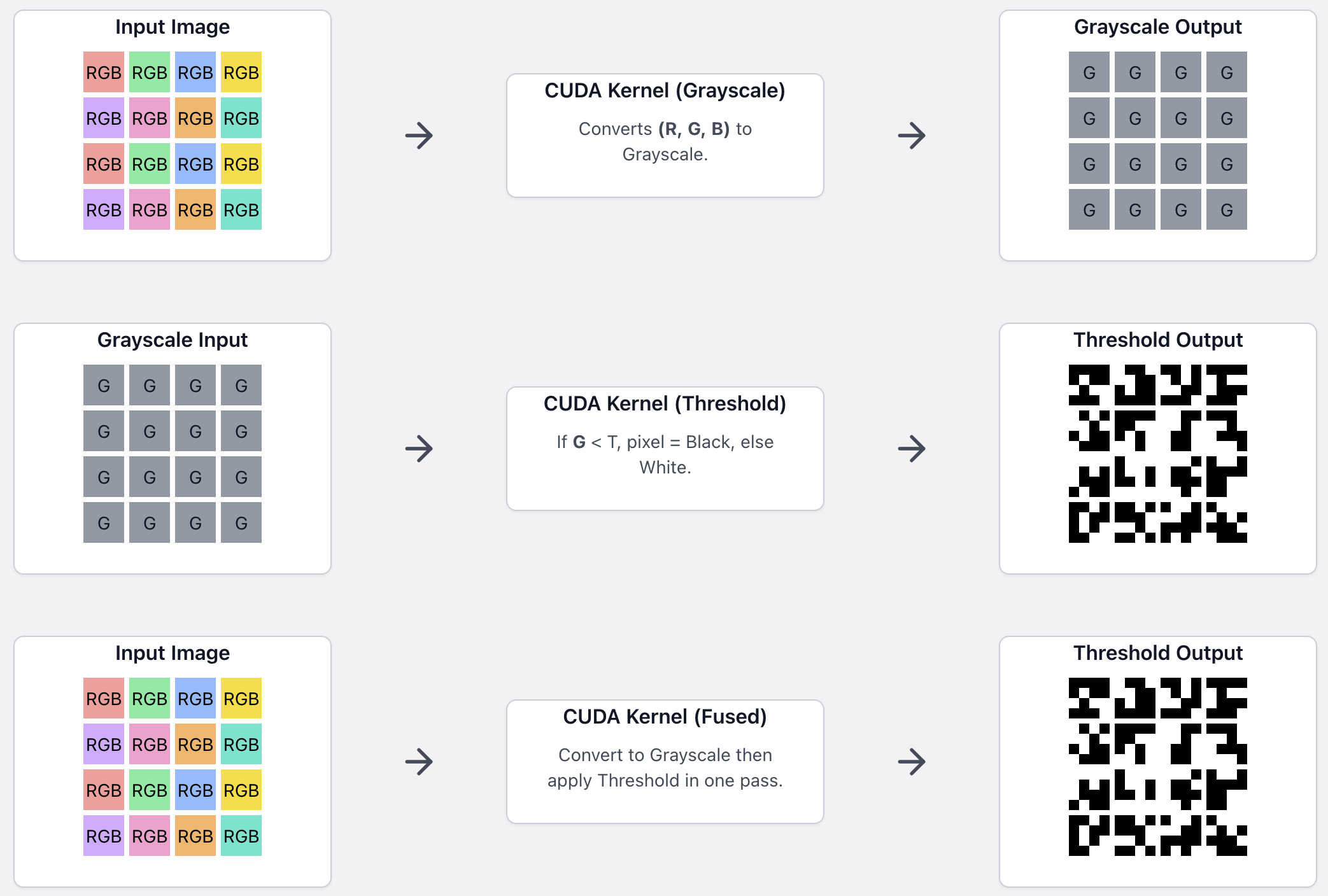
Each small rectangle is a patch handled by a launched kernel. For each kernel execution example, all patches are launched in parallel.
Broadly speaking, kernel fusion refers to implementing kernels that do more work by "fusing" together multiple kernels. To expand on the grayscale example, imagine we would additionally have a kernel that thresholds all pixels with a value smaller than a constant. If we fused them, we would apply the thresholding on the grayscaled pixel in our code, and write the final result in one function call. If we launched the grayscale kernel, waited for it to finish, and then launched the threshold kernel on the grayscaled image, we would lose throughput for multiple reasons:
- We would load the entire image once for the grayscale kernel, store it, then load it again for the thresholding, and store the final result. The load/store operations are much slower on hardware than the actual computation that we do.
- We double the memory usage by storing the intermediate results for grayscaling.
- Kernel launches themselves add overhead. If your code has to launch many short kernels, this can impact performance.
Kernels and PyTorch
When writing PyTorch programs, the default mode of execution is eager, which means that all functions are immediately executed when they are encountered in code, with no automated optimizations. Consider this simple PyTorch script:
x = torch.exp((x * scale) ** 2)
It might be surprising if you are not familiar with the details of eager mode to find out that this line of code will result in 3 memory allocations2 of the size of x and 3 kernel launches. The multiplication by scale, the squaring and the exponentiation will each result in one kernel call and memory allocation.
Torch.compile
While eager execution has its advantages, it is often wasteful in terms of both memory and compute. This is the reason tools like torch.compile have been developed, to offer an automated way to fuse kernels in PyTorch code. Torch compilation is definitely a powerful tool that can significantly speed up your code. That being said, certain optimizations are still out of reach for current compilers, such as FlashAttention. It seems that fused gated MLPs are currently also part of this class of optimizations, since we did not measure any improvements over the eager cuBLAS+Unsloth (we will clarify what this refers to in the Benchmarking section) approach when compiling the PyTorch gating module in our repo.
Our approach
In this section, we will give a high-level overview of the solution we came with to fuse some of the MLP computation. To recap, a Transformer MLP might look like this in PyTorch code:
def mlp(x: torch.Tensor, weights_upscale: torch.Tensor, weights_downscale: torch.Tensor, weights_gate: torch.Tensor, act_fn: Callable) -> torch.Tensor:
    up_scaled_x = x @ weights_upscale # linear projection
    gate_values = x @ weights_gate # linear projection
    gated_up_scale = up_scaled_x * act_fn(gate_values) # element-wise product with gate values passed through activation
    result = gated_up_scale @ weights_downscale # linear downscaling
    return result
What we have currently worked on are the 2-4 lines of code. The algorithm can be summarized as follows:
- Concatenate the upscaling weights and gating weights on the second dimension (i.e. add extra columns), such that we can compute both the up scaled and the gating values in one matrix multiplication. This is a standard optimization used in many LLM projects. The main difference is that we interleave columns, with even positions corresponding to upscaling weights and odd positions to gate weights. This is helpful, because our kernel can only compute a small patch of both the up-scaled weights and the gating values. By grabbing the odd and even columns, we can compute the local gated patch.
- Compute the GEMM (General Matrix Multiplication). It is very important for our approach to be able to directly work on the result of the matrix multiplication and manipulate its shape, therefore we cannot use highly efficient, but closed source kernels like cuBLAS. For this purpose, we wrote a custom GEMM kernel.
- Each CTA now holds a patch of the final linear projection. To compute the gated linear unit (line 4), we take all odd columns from the patch, apply the activation function on them, and multiply them by the even columns.
- We write the result to
gated_up_scale.
By doing this, we only need enough memory to store a Tensor the size of gated_up_scale, and we fuse the inefficient gating multiplication in the GEMM kernel. This cuts the memory usage by more than two thirds compared to our PyTorch code above. Before looking at some benchmarks, let's quickly discuss other existing solution for efficient MLPs.
Triton kernels
Several Triton kernels for the fourth line of code in our mlp function are available, such as Liger kernels [7] or UnslothAI [8]. While certainly much more efficient than just eager PyTorch code, they still require extra memory for storing the up_scaled_x and gate_values. We can save some memory by writing gated_up_scale over either of these two Tensors, but that is still twice as much memory as our approach. Nevertheless, in our benchmarks we use a cuBLAS kernel for computing the matrix multiplications, and Unsloth kernels for the activation, as they are otherwise highly efficient.
Furthermore, in this repo there are Triton fused kernels for both the forward and backward passes of the GEMM and gate operation.
CUDA kernels
A similar approach to our gated MLP kernel exists in the TensorRT-LLM repo here. At a high-level the kernels are conceptually similar, in that they both fuse the gating computation with the GEMM. The similarities stop here, as the one from TensorRT-LLM is written and very optimized for the Hopper architecture, and used only for FP8 MLPs. The fusing itself also does not use the odd-even column scheme we employ, instead they do two separate GEMMs for the weights. In any case, we see this as a confirmation that fusing these kernels is a promising approach. We did not benchmark against their kernel, because our code is written for Ampere, since that is the hardware available for us (A100).
Additionally, the xformers library includes a fused implementation that utilizes the DualGemm class from the Nvidia CUTLASS library.
Benchmarks
Before deep diving into low-level details, we wanted to show the performance of our kernel when compared to an optimized way of computing the MLP in PyTorch:
def forward(self, C):
    # X and W are the inputs and concatenated weights
    torch.mm(self.x, self.w, out=C)
    # self.N is 2 x D_up
    return swiglu_fg_kernel(C[:, :self.N//2], C[:, self.N//2:])
The torch.mm call will call a cuBLAS optimized kernel, and swiglu_fg_kernel corresponds to the Unsloth kernel, with the modification that it overwrites the second argument with the result, to save on memory. We call this implementation cuBLAS+Unsloth throughout our blog, since it uses the cuBLAS GEMM kernel and the gate Triton kernel from UnslothAI. The code for the benchmarks is provided in the GitHub repo. We use the Triton benchmarking module to measure the TFLOP/s achieved by the above code and our kernel. All benchmarks are run on an A100 80GB card, with bf16 precision for all tensors. We also report the results for the Triton kernel and xformers implementations.


TFLOP/s for different sizes of Llama models and sequence lengths.


TFLOP/s only for our kernel and cuBLAS+Unsloth.


Memory usage for different sizes of Llama models and sequence lengths.
Our kernel underperforms in terms of TFLOP/s, achieving between 95-98% of the cuBLAS+Unsloth approach, but we can ease the memory pressure by half. This can result in elevated throughput for inference workloads, as the memory saved could be used for expanding the KV cache, for example.
We also note that the difference in terms of compute is mostly explained by the difference in performance between our GEMM code and the extremely optimized cuBLAS kernel for the A100. Our claim is based on the observation that the performance gap between cuBLAS and our standalone GEMM code is generally larger than the gap between our complete kernel and the cuBLAS+Unsloth code. The table below shows the ratio between the TFLOP/s of our kernel GEMM code and cuBLAS for the GEMM column, and the Full column refers to the ratio of our complete kernel and cuBLAS+Unsloth. We see that for most model sizes and token counts the gap between the GEMM computations is higher, and in all cases the ratios are closely matched.
| Tokens | 8B | 70B | 405B | |||
|---|---|---|---|---|---|---|
| Full | GEMM | Full | GEMM | Full | GEMM | |
| 1024 | 102.79% | 101.59% | 96.03% | 95.74% | 95.54% | 95.80% |
| 2048 | 97.40% | 96.23% | 96.64% | 96.19% | 95.55% | 96.12% |
| 4096 | 98.42% | 97.30% | 96.04% | 95.52% | 95.93% | 96.24% |
| 8192 | 97.71% | 96.55% | 95.77% | 95.24% | 95.67% | 95.85% |
| 16384 | 97.29% | 95.96% | 95.93% | 95.50% | 95.85% | 95.99% |
| 32768 | 97.30% | 95.99% | 96.16% | 95.72% | 95.81% | 96.11% |
| 49152 | 97.30% | 96.02% | 96.16% | 95.75% | 95.75% | 96.05% |
| 65536 | 97.30% | 95.99% | 96.13% | 95.80% | 95.76% | 96.05% |
In principle, any GEMM kernel for Ampere should be amenable to fuse the gated linear unit in the way we do in our code, since the mma instruction will result in similar shapes for the slices of data threads act on. Therefore, we see this as a positive result, in the fact that with more optimized GEMM code it should be possible to match or even exceed the performance of cuBLAS+Unsloth in terms of TFLOP/s. We will explain this in more detail in the low-level section of our blog.
Impact on model capabilities and correctness
To check the correctness of our model, we ran numerical tests where we measured the difference between the outputs of our kernel and the PyTorch code, using matrices initialized with Kaiming initialization, which is the default option for PyTorch weights. All of the tensors are kept in bfloat16 precision. We use square matrices with the shape indicated by the MNK column. We run 100 iterations of random initializations to compute the mean and standard deviation of each statistic. We report the results in the following table:
| MNK | Max Abs Diff (Mean ± Std Dev) | Mean Abs Diff (Mean ± Std Dev) | Relative Diff (Mean ± Std Dev) |
|---|---|---|---|
| 1024 | 3.91e-06 ± 5.64e-07 | 8.08e-08 ± 2.96e-10 | 3.71e-03 ± 1.41e-05 |
| 2048 | 2.02e-06 ± 4.11e-07 | 4.09e-08 ± 1.13e-10 | 3.74e-03 ± 6.35e-06 |
| 4096 | 1.29e-06 ± 4.44e-07 | 2.08e-08 ± 1.16e-11 | 3.80e-03 ± 9.88e-06 |
| 8192 | 7.25e-07 ± 2.13e-07 | 1.04e-08 ± 0.00e+00 | 3.86e-03 ± 4.34e-19 |
| 16384 | 4.77e-07 ± 0.00e+00 | 4.98e-09 ± 0.00e+00 | 3.81e-03 ± 0.00e+00 |
| 32768 | 2.72e-07 ± 6.10e-08 | 3.46e-09 ± 0.00e+00 | 4.34e-03 ± 0.00e+00 |
| 65536 | 1.69e-07 ± 2.76e-08 | 1.68e-09 ± 0.00e+00 | 4.22e-03 ± 0.00e+00 |
However, it is possible to degrade model performance even with small numerical errors, due to the compounding effects over the many layers models have. Therefore, we measure the performance of a Llama 8B model on three popular benchmarks, with and without our kernel.
| Benchmark | MLP kernel | MLP eager |
|---|---|---|
| MMLU-Pro (0-shot) | 44.37 | 44.24 |
| EvalPlus (0-shot) | 61.6 | 60.4 |
| GPQA (0-shot) | 33.71 | 31.92 |
We observe no degradation in terms of score across reasoning tasks, code and math problems, or the general knowledge required for some of the MMLU-Pro categories.
Inference
First of all, inference engines usually split the process of generating a response to a given request in 2 phases: prefilling and decoding. Prefilling is the first phase, in which the model receives the full user prompt. The prompt is passed through the entire model, and at each layer, all the keys and values are saved in the KV cache. The decoding phase refers to the process in which the model generates new tokens. After the first sampled token in the prefill phase, the model will only pass the currently generated token through the query projection and the MLP for each layer, as it can fetch the keys and values from the KV cache to perform self-attention.
This would hint that our kernel would mostly be useful for the prefill phase, as that's when we can expect the peak memory usage for MLP activations. Considering the sequence length of a prompt, the dimension used for queries and keys, and the up-scaling dimension, a full decoder layer uses memory for self-attention (queries, keys, values and output) and memory for the MLP (up-scale, gate values up-scale, gated result, down-scaled output). By using only memory for the first half of the MLP, we would reduce memory usage per-layer by a factor of around 3 for activations, assuming an efficient attention kernel, such as FlashAttention. The saved memory could then be used for larger KV caches or models.
On the other hand, modern inference engines also use chunked prefill to further improve latency. During chunked prefill, instead of splitting the computation in two phases, the model will always be served a chunk of tokens that can be either part of an user prompt, or used for decoding other requests. The advantage of this technique is that decoding is no longer bottlenecked by potentially very long prefills, as can be seen in the picture below, taken from an Nvidia blog.
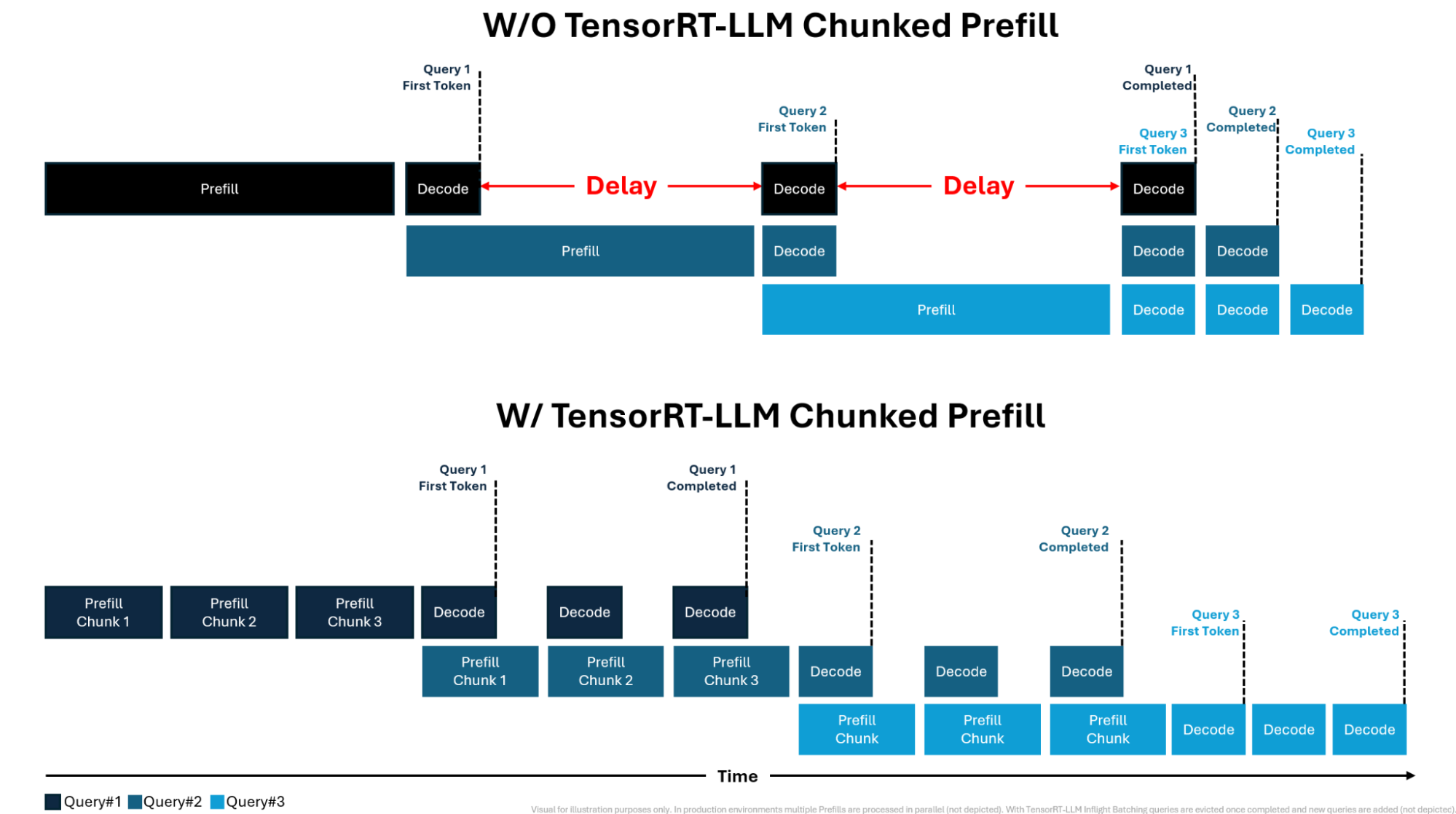
Chunked prefill illustrated, from Nvidia.
A side-effect of chunked prefill is that the memory used by activations drops even lower than in "classic" prefill-decode inference. As now the model will only be fed one chunk at a time, we only need activation memory for one chunk. Inference engines that implement chunked prefill use or tokens for a chunk, so we can actually exactly compute the amount of memory we save for a given model, per deployment.

The extra tokens are estimated by dividing the total saved memory by the required memory of a key and value for all layers of a model.
We plot in these graphs the amount of tokens that we can further add to the KV cache when reducing the activation memory per chunk with a chunk size of . This value is fixed per model deployment, since it only depends on the chunk size and model configuration. The stronger dependence on model configuration is also the reason why the graphs have irregular patterns. The gains are more modest in this scenario, given the small chunk sizes. Nonetheless, they can still help squeeze more value out of existing deployments. Notably, Gemma 2-27B has the highest up-scaling factor of , and we can see it leads to the largest potential increase in KV cache memory.
A closer look
So far, we kept the blog post at a reasonably high-level in terms of details. The next parts of the blog post are all dedicated to low-level details of our kernel that we think might be relevant, and at the very least interesting.
CuTe
CuTe is a collection of low-level templates from the Nvidia CUTLASS library that is very handy for writing kernels. We extensively use CuTe throughout our kernel, since it's very helpful with computing the shapes of various tensors used throughout a GEMM kernel.
Tiling with CuTe
One of the main things that CuTe simplifies is tiling tensors. For example, to obtain the tile of the A matrix that the current CTA (Cooperative Thread Array, also known as threadblock) acts on, one can write:
// (M,K) row-major matrix in global memory
Tensor mA = make_tensor(make_gmem_ptr(A), make_shape(M, K), make_stride(K, 1));
// _ refers to selecting all indexes on the K dimension
auto cta_coord = make_coord(blockIdx.x, blockIdx.y, _);
// tile shapes
auto cta_tiler = make_shape(bM, bN, bK);
// selects bM and bK as tile dimensions, and uses cta_coord to select the rows and columns corresponding to this CTA
Tensor gA = local_tile(mA, cta_tiler, cta_coord, Step<_1, X, _1>{});
In the above example, mA corresponds to the large matrix and is initialized with a GMEM pointer and the appropriate shape and stride. The CTA-level tile gA will have shape (bM, bK, k), where bM and bK are the dimensions used for a tile, and k is the amount of times the tile has to be repeated in the dimension to completely fill a row. Furthermore, the offset with regards to the global memory pointer is automatically computed by CuTe. This makes indexing easier to follow, especially when working with thread-level Tensors, as their shapes can get convoluted even with the simplifications provided by CuTe. For example, the thread-level tensor used for indexing into shared memory when copying the final gated result is a rank-3 tensor of shape (2, 4, (2, 2, 2)) 4 with stride (512, 2048, (8, 16, 32)).
However, the CuTe approach can have some drawbacks once we start trying to do some more unusual manipulation on the shapes. In particular, when we write our shapes for the GEMM part, the final result of the GEMM will be a tile of shape (bM, bN). After the gating, we will need to reduce this to a (bM, bN/2) tile, with the appropriate changes to the strides. In principle, it is possible to do this by carefully constructing new Tensors in code from the original tile returned by CuTe. This is the first solution we tried, but we found it to be very difficult to scale to all the Tensors used throughout the kernel, besides also being an unflexible approach in terms of varying the tile shapes and Atoms used. We therefore sought to find an approach where we get the correct Tensor shapes by using the same pipeline we apply on the GEMM Tensors. This would have the advantage of allowing us to reuse the GEMM tiling code to obtain the gating tile, and it would also be more robust, since in this case we would rely on the same CuTe functions used throughout the kernel.
CuTe Atoms
Atoms in CuTe can be thought of as the basic building block for constructing thread-level Tensors and calling the relevant PTX instructions. They are mostly defined by an Operation and Traits struct. Operation handles calling the relevant PTX instruction and directly receives the raw pointers for the registers, while Traits contains information such as the Layout of the Tensor or the data type used. The common practice for CuTe is to build thread-level Tensors that usually have the shape (ATOM, ATOM_M, ATOM_N), where ATOM is the shape on which the PTX code will be called, and ATOM_M refers to how the Atom is tiled on the M dimension (similarly for N).
For example, if we would use a vectorized load copy instruction on half precision data, we would expect a shape like ((8, 1), tiled_m, tiled_n):((1, 0), stride_m, stride_n). The (8, 1):(1,0) Atom means that we will load 8 numbers across whichever is the major dimension, which is exactly 128 bits.
In our case, we are interested in changing the shape of the MMA Atom to reflect the halved column dimension after the gating operation. Since we only need to change the shapes and do not care about the PTX code, we will skip inspecting the Operation struct. So, let's take a look at the code for the Atom Traits that we use in our GEMM:
template <>
struct MMA_Traits<SM80_16x8x16_F32BF16BF16F32_TN>
{
  using ValTypeD = float;
  using ValTypeA = bfloat16_t;
  using ValTypeB = bfloat16_t;
  using ValTypeC = float;

  using Shape_MNK = Shape<_16,_8,_16>;
  using ThrID   = Layout<_32>;
  using ALayout = Layout<Shape <Shape < _4,_8>,Shape < _2,_2,  _2>>,
                         Stride<Stride<_32,_1>,Stride<_16,_8,_128>>>;
  using BLayout = Layout<Shape <Shape < _4,_8>,Shape <_2, _2>>,
                         Stride<Stride<_16,_1>,Stride<_8,_64>>>;
  using CLayout = Layout<Shape <Shape < _4,_8>,Shape < _2,_2>>,
                             Stride<Stride<_32,_1>,Stride<_16,_8>>>;
};
This corresponds to a warp-level mma instructions for the Ampere architecture, that computes the product of a tile from with a tile from B, and holds the layouts for the entire warp. The way to interpret these layouts is that the second rank corresponds to the elements each thread will provide for the mma, and the first rank represents the thread layout (note that it is always exactly in size, which is a warp). Taken together, the layouts represent a mapping from the (Thread, Value) space to the Tile indices.
To get a clearer picture of what this means, let's inspect ALayout. First, we can see that each thread will use a value of shape (2, 2, 2) and size . This makes sense if we take this in the context of the A tile, which is , and the fact that this is executed at warp-level, which has threads. That would imply each thread needs to provide values from the A tile. Furthermore, we can look at the PTX documentation to get a visual intuition of how the threads are mapped to their respective fragments of the tile:
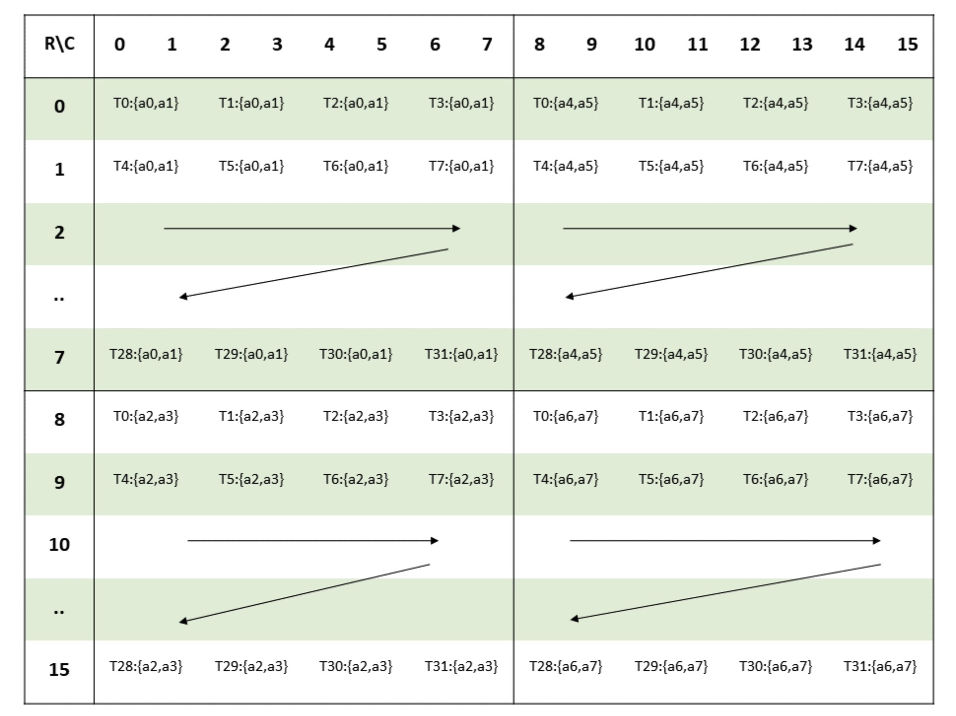
Image from PTX documentation.
Let's focus on thread , we can see that it handles the upper left corner of each tile in the matrix fragment. Each such corner corresponds to a pair of values, and this adds up to the total of values it provides to the mma instruction.
Next, let's understand how we can use Atoms in CuTe kernels to build larger tiles. The above Atom only works at the level of one warp and with only small tiles, but that is very unlikely to be sufficient to achieve good performance. In this case, there are 2 ways we can increase the amount of work a kernel does: (1) using more threads in CTAs and (2) increasing the amount of values each thread handles (thread coarsening). CuTe provides a very straightforward way to do both:
// 16x8x16 mma from above
TiledMMA mma = make_tiled_mma(SM80_16x8x16_F32BF16BF16F32_TN{},
        Layout<Shape<_2, _2>>{}, // (1) larger CTA
        Tile<_64,_32,_32>{});    // (2) thread coarsening, MxNxK shape
In line 2, we tile two times across both and dimensions by increasing the number of warps in our CTA to a total of , which corresponds to threads. This also means that so far we can compute a final result, since we repeat the tile twice. On line 3, we coarsen each thread, by doubling how many elements each thread has to handle. Importantly, CuTe does not always throw a compile error for incorrect values in the tile. For example, using Tile<_64, _8, _32> would work, even if it doesn't make sense. This detail can lead to confusing runtime errors, and is especially important for the way we will solve the gate tile issue.
Computing the gated result
Before showing how we can obtain the required Tensor shapes, let's quickly take a look at how we compute the gated result. Remember that we store our weights by using the odd and even columns for the two up-scaling matrices. In particular, we make sure that corresponds to the same column in the original weight matrix, e.g. column 1 is equivalent to the first column of the gate weights, and column 0 is the first column of the up-proj weights. Using this, we simply write:
CUTE_UNROLL
for(int j = 0; j < MMA_N; ++j) {
  CUTE_UNROLL
  for(int i = 0; i < MMA_M; ++i) {
    tCrC_gate[make_coord(0, i, j)] = cast_mmaresult<TC>(
      tCrC[make_coord(make_coord(0, 0), i, j)] *
      silu(tCrC[make_coord(make_coord(1, 0), i, j)]));

    tCrC_gate[make_coord(1, i, j)] = cast_mmaresult<TC>(
      tCrC[make_coord(make_coord(0, 1), i, j)] *
      silu(tCrC[make_coord(make_coord(1, 1), i, j)]));
  }
}
Let's also take a look at the mapping of threads to values used by mma for the C matrix:
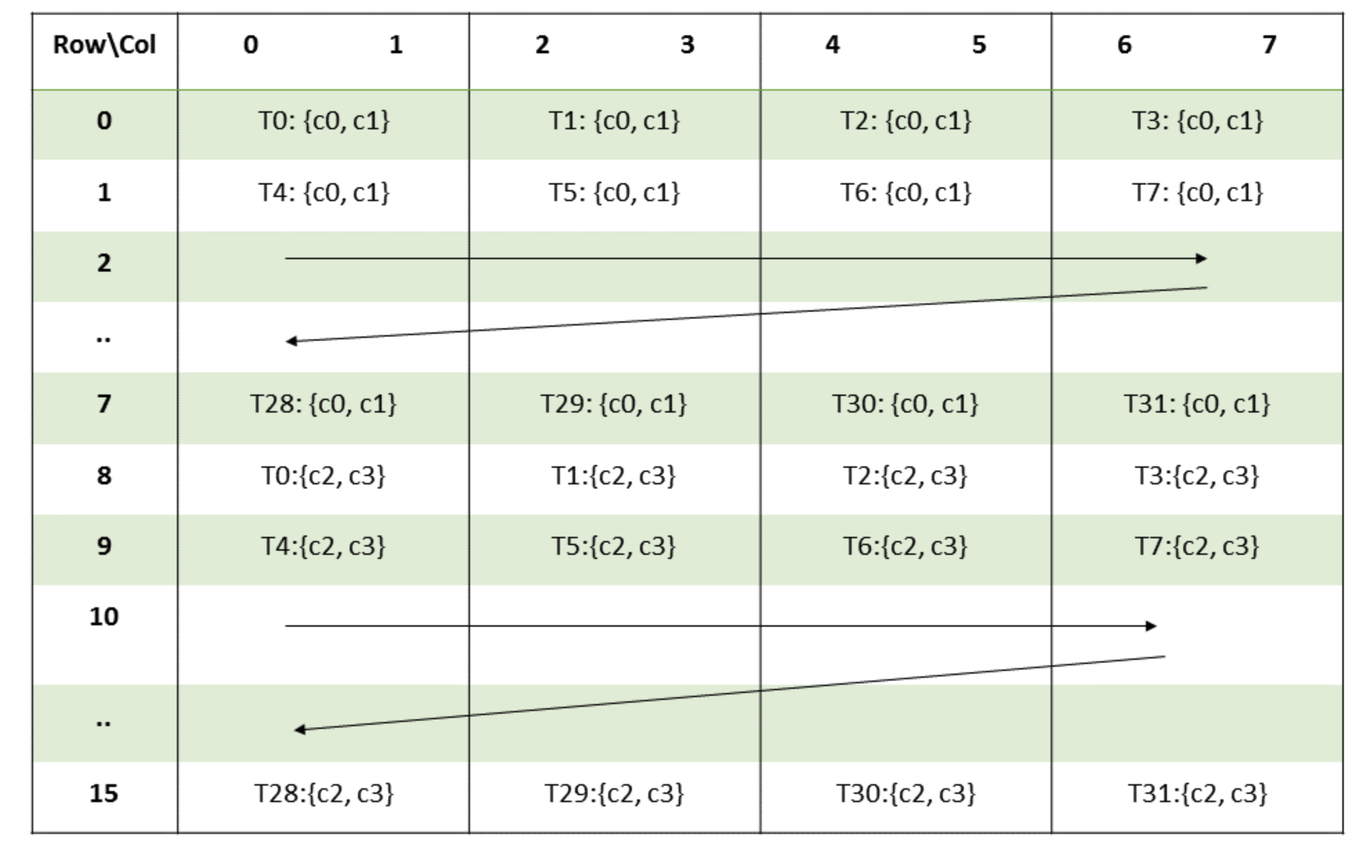
As we can see, each thread will always hold a pair of two elements. Furthermore, we know that from the way we do tiling that c0 will always be an even column and c1 an odd column. This is the key reason we can be sure our algorithm is correct, as this structure generalizes to all warps. It only remains to see how we can construct the tCrC_gate Tensor in a clean fashion.
Custom MMA Atom
Finally, we can explain our solution. What we did is to define this Traits Atom for an imaginary MMA:
  template <>
  struct MMA_Traits<SM80_16x4x16_F32BF16BF16F32_TN_GATED>
        : MMA_Traits<SM80_16x8x8_F16F16F16F16_TN>
  {
    ...
    // 4 is very important here, since we reduce the atoms on the feature (N) dimension
    using Shape_MNK = Shape<_16,_4,_16>;
    using ThrID   = Layout<_32>;
    // A and B don't really matter, this atom is useful only for creating the right shapes for the C layout
    ...
    // the C layout suggest the (2) atoms used for the merging
    // and the strides are changed to make sense in terms of the new numel
    using CLayout = Layout<Shape <Shape < _4,_8>, _2>,
                             Stride<Stride<_16,_1>,_8>>;
  };
Because we are only interested in using this Atom to work on the result of the GEMM, we can leave the A and B layouts unchanged from the earlier struct. The change is relatively easy to understand, we reduce the value for each thread from (2, 2) to (2), as we will multiply each odd-even pair to do our gating. We also have to adapt the stride values to our smaller layout. Relating to the earlier figure of the C matrix, this is equivalent to reducing each pair to just one element, through the gating operation.
We can now keep the code almost completely unchanged and apply the same transformations we do to obtain the thread values for the C matrix during the GEMM, as they are guaranteed to be applied in the same way, but with our corrected CLayout. For example, the fragments are obtained in essentially the same way:
// for the GEMM
Tensor tCgC = thr_mma.partition_C(gC);
Tensor tCrC = thr_mma.make_fragment_C(tCgC);
// for the gating
Tensor tCgC_gate = thr_mma_gate.partition_C(gC_half);
Tensor tCrC_gate = thr_mma_gate.make_fragment_C(tCgC_gate);
// and so on
As can be seen in the code snippet, there are still some small changes we need to make. In particular, we need to ensure we adjust some strides before calling the kernel, since our rows are shorter than what a GEMM kernel would expect. If we use thread coarsening, we also must be careful in the final Tile<> definition to account for the halved N dimension. Regardless, we find that handling these details outside of the kernel code is significantly easier to follow than directly manipulating Tensor shapes and strides in the kernel.
Closing thoughts
Can this be extended to any GEMM kernel?
We earlier claimed that any efficient Ampere GEMM kernel should be amenable to fuse gating in a similar manner. The reason for that is the mma instruction, more exactly the way the C matrix is held by each thread. As we have mentioned in the low-level section, all threads in a warp will hold pairs of elements. If it's possible to determine the parity of each element of the pair, a similar algorithm to what we propose should be achievable, which we think is the case for most (if not all) efficient kernels.
The reason we specify Ampere is that the algorithm hinges on the particular structure of the C matrix. However, in general mma-like instructions tend to hold multiple adjacent values per thread, which suggest a similar odd-even scheme should be possible for other architectures. For warp-level instructions that hold just one value per thread, warp shuffling could be used to exchange data intra-warp.
Future directions
So far, we have focused only on the first half of the MLP computation. More so, our optimization concerns just the forward pass, as for a backward pass it's generally more efficient to store intermediary results anyway, and therefore our kernel would achieve lower throughput. We are interested in studying the possiblity of fusing the entire MLP in a single kernel. A more immediate goal would be to improve our current kernel, mainly to further bridge the gap to cuBLAS performance.
References
[1]. Flash Attention, Dao et. al: https://arxiv.org/abs/2205.14135
[2]. Longformer: The Long-Document Transformer, Beltagy et. al: https://arxiv.org/abs/2004.05150
[3]. Mamba: Linear-Time Sequence Modeling with Selective State Spaces, Gu et. al: https://arxiv.org/abs/2312.00752
[4]. Resurrecting Recurrent Neural Networks for Long Sequences, Orvieto et. al: https://arxiv.org/abs/2303.06349
[5]. Transformers are SSMs: Generalized Models and Efficient Algorithms Through Structured State Space Duality, Dao et. al: https://arxiv.org/abs/2405.21060
[6]. GLU Variants Improve Transformer, Noam Shazeer: https://arxiv.org/abs/2002.05202
[7]. Liger Kernel: Efficient Triton Kernels for LLM Training, Hsu et. al https://arxiv.org/abs/2410.10989
[8]. UnslothAI, Han et. al: https://github.com/unslothai/unsloth
Credits
Blog background image generated with DALL·E 3.
- Here we should also note that the discussion for warps is also more nuanced, since we skipped talking about warp divergence.↩
- In practice, PyTorch uses its own CUDA memory allocator. A simplified way to look at it is that when a tensor frees memory, PyTorch doesn’t immediately return it to the GPU. Instead, it holds onto the memory for reuse, reducing the overhead associated with
cudaMallocandcudaFreecalls. Therefore, scripts similar to this one might not actually result in increased total memory usage, and will (probably) always use less than times the memory ofx, since thex * scalingterm can be freed after the squaring operation.↩ - This is computed as the ratio , where is short-hand for the up-scaling dimension. This further reduces to . Since we have with in practice, we can simplify this to , which is lower bounded by in the limit, and upper bounded by for . This translates for gains per layer as the up-proj dimension gets larger. If we assume some more memory optimizations, like overwriting the queries with the outputs and the up-scaled MLP inputs with the gating result (for example), we can reduce the memory requirement to . Using the same series of calculations we would arrive at a gain.↩
- We are not entirely sure why CuTe doesn't reduce this to a
(2, 4, 8): (512, 2048, 8)layout, but this further reinforces why trying to directly operate on the raw layouts is a bad idea.↩