The BGV fully homomorphic encryption scheme

This is a sister blogpost to the previous one about a similar scheme (BFV) and it's part of the series that covers fully homomorphic encryption techniques and applications.

Introduction

$\gdef\can #1{\|#1\|^{\text{can}}}$

In this blogpost we will focus on the encryption, decryption, relinearization and the noise analysis of the Brakerski, Gentry, Vaikuntanathan (BGV) fully homomorphic encryption scheme. A Python implementation of the aforementioned will be provided.

DISCLAIMER: This toy implementation is not meant to be secure or optimized for efficiency. It's for educational purposes only, and for us to better understand the inner workings.

What to expect from this blogpost?

1. We briefly describe the motivations of fully homomorphic encryption.
2. We present the BGV scheme.
3. We offer a Python implementation for the BGV scheme, for educational purposes.

Now, let's make a short, informal, tour before starting. Fully homomorphic encryption (FHE) allows us to perform computation on encrypted data. While there are a few cryptographic schemes to achieve this, in this blogpost we explore the BGV scheme.

Firstly, this scheme allows us to encrypt messages into ciphertexts. Intuitively, a message is hidden in a ciphertext if there is no way to get to retrieve the original message from its encryption. To an attacker that sees a ciphertext, that ciphertext should look like "random garbage". In order to achieve this we hide the message by "masking" it with some noise. We say it's hard for an attacker to retrieve a message from its ciphertext if doing so is at least as hard as solving a computationally unfeasable problem. The problem the security of the BGV scheme is based on is called the Ring Learning with Errors problem.

Secondly, the scheme allows us to perform arithmetic operations (additions, multiplications) using noisy ciphertexts. However, we will encounter some problems along the way, such as the noise increasing after computations, or the size of the resulting ciphertext increasing. We'll see how to handle these using modulus switching (for the former) and relinearization (for the latter).

This post will get a bit mathematical, so before starting we introduce some notation. Any other notation will be defined when introduced.

Notations:

• $m, m', m^*$ - messages.
• $c, c', c^*$ - ciphertexts. If ciphertexts have more components, we denote the components with indices: $c = (c_0, c_1)$
• $\lambda$ - Security parameter.
• $\mathbb Z_q$ - the set of integers from $(-q / 2, q / 2]$
• $R$ - Ring.
  • Ex: $\mathbb Z$ - the integers.
  • Ex: $\mathbb Z[X] / (X^n + 1)$ - the quotient polynomial ring with integer coefficients: .
• $R_q$ - Ring modulo the ideal generated by $q$.
  • Ex: $\mathbb Z_q$ - the integers mod $q$.
  • Ex: $\mathbb Z_q[X]/ (X^n + 1)$ - the quotient polynomial ring with coefficients being integers in $(-q / 2, q / 2]$.
• $[a]_q$ - $a \bmod q$, coefficients centered in $(-q / 2, q / 2]$. When applying $[\cdot ]_q$ to a polynomial we mean to apply it to all its coefficients individually. When applying $[\cdot]$ to a vector of elements, we mean to apply it to each element individually. So $[(a, b)]_q = ([a]_q, [b]_q)$. We give the similar treatment to reduction $\bmod q$ operation
• $\chi = \chi(\lambda)$ - Noise distribution, parametrized by $\lambda$ (usually Gaussian).
• For simplicity, when we say we sample a polynomial from some distribution (or a polynomial comes from some distribution) we mean that its coefficients are sampled independently from that distribution.
• $e \leftarrow \chi$ - An element $e$ sampled from the distribution $\chi$
• $a \xleftarrow R S$ - An element sampled uniformly from a set $S$
  • Ex: $a \xleftarrow R R_q$ An element $a$ sampled uniformly from the ring $R_q$
• $a \cdot b$ denotes the multiplication of 2 elements from the ring $R_q$
• $ta$ denotes the multiplication of coefficients of $a \in R_q$ by some scalar $t$.

Fully Homomorphic Encryption (FHE)

Before defining fully homomorphic encryption, let's look at some applications of it to get a better intuition:

1. Outsourcing storage and computations

• A company wants to use a cloud provider to store data and do computational heavy lifting.
• Task: The company wants to use the information (for example: to do machine learning, extract statistical properties) without locally retrieving it (defeating the purpose of using the cloud company services). Furthermore, the company doesn't want the cloud provider to see the sensitive data.
• Solution: Using homomorphic encryption, the company can encrypt and send the data to the cloud provider and then the cloud provider can process the information (as requested by the company) in the encrypted form, without learning anything about the data.
• Ex: finance, medical apps, consumer privacy in ads.

2. Private queries

• A client wants to retrieve a query against a large database held by a provider.
• Task: The client wants to retrieve a query without the database provider learning the query.
• Solution: Using homomorphic encryption the client can encrypt the index of the record and then the database can use this encrypted index to fetch (the comparison operation can be done using FHE) and return the encrypted result to the client. Finally, the client can decrypt the record.

3. Private set intersection

• A client and a server each has a set of elements. The client wants to know which elements from its set are in the server's set.
• Task: The client wants to find out the intersection of its elements and the server's, without the server learning anything about the client's elements and vice versa.
• Solution (Very simplified): They translate the comparison operation into a subtraction ($x = y \Rightarrow x - y = 0$). The client encrypts its elements and sends them to the server. Then, the server evalutes these subtractions homomorphically. Because the result of the subtraction is an encrypted result, the server learns nothing. Then the server sends the comparison results back and the client decrypts the results. We have a longer, more in-depth blogpost about it here. Happy reading!
• Examples: Client: user contacts, Server: whatsapp contacts; Client: own passwords, Server: database with breached passwords.

Intuition

• A user has an arithmetic function $f$ and some inputs $(m_1, ... m_n)$.
• He wants to compute $m^* = f(m_1, ... m_n)$ but instead of computing it directly, he wants to encrypt $(m_1, ... m_n) \to (c_1, ... c_n)$ and do the computation on the ciphertext, obtaining a result which eventually decrypts to $m^* =f(m_1, ... m_n)$.
• It's helpful to view the functions as tree of operations. For example (taken from the BFV blogpost): $f(m_1,m_2,m_3,m_4)= (m_1 \times m_2 + m_3) \times m_4$

Homomorphic Encryption -- Definition
Let $(\text{KeyGen}, \text{Enc}, \text{Dec}, \text{Eval})$ be a tuple of procedures.
Let $f \in \mathcal F$ be a function in a family of functions. This function can also be written as a circuit from a family of circuits $C \in \mathcal C$.

• $(sk, pk) \gets \text{KeyGen}(1^\lambda, 1^d)$ - key generation, $\lambda$ is a security parameter, $d$ is a functionality parameter (degree of the polynomial or depth of the circtuit).
• $c_i \gets \text{Enc}(pk, m_i)$ - Encryption of a message $m_i$ -- known as fresh ciphertexts.
• $c^* = \text{Eval}(pk, f, c_1, ... c_n)$ - Evaluate the function $f$ on the ciphertexts -- known as evaluated ciphertexts.

Correctness
We require the (FHE) scheme to correctly decrypt both fresh and evaluated ciphertexts: $\text{Dec}(sk, c^*) = m^* = f(m_1, ..., m_n)$

In the image above, the user with the laptop is interested evaluating a certain circuit on its data $m$. Therefore it sends its data, encrypted, to the cloud so that the cloud computes the circuit. By correctness, the user indeed gets the circuit applied on its data $m$.

Circuits?
The two important operations we care about are addition and multiplication, because with them we can construct any arithmetic operation! Homomorphic encryption schemes started out by encrypting bits, so the equivalent operations for additon and multiplication on bits, xor and and are used.

To convey the fact that a circuit supports both xor and and usually a nand gate is used, because nand gates are composed by 1 multiplication and 1 addition and they are logically complete (you can build any circuit with them). $\text{nand}(a, b) = a \times b + 1 \bmod 2$

By extending to multiple bits, with the gates we discussed above you can represent any computation using boolean circuits.

HE can be classified based on the type of functions $f$ that it supports:

• Partially homomorphic encryption
  Given $\text{Enc}(m_1)$, and $\text{Enc}(m_2)$ you can do limited operations (either additions or multiplications)
• Somewhat (leveled) homomorphic encryption
  Given $\text{Enc}(m_1), ..., \text{Enc}(m_n)$ you can compute $\text{Enc}(f(m_1, ... m_n))$ where $f$ is a polynomial of a limited degree. One can do limited number of multiplications (Circuits of a maximum depth).
• Fully homomorphic encryption
  One can do unlimited multiplications and additions.

The community put a lot of effort into the analysing FHE schemes: finding good parameters, finding software and hardware optimizations, coming up with possible attacks and adjusting the schemes against them. An interesting read is the homomorphic encryption standard, which compiles good practices and techniques for developing and using existing schemes.

Ring Learning With Errors (RLWE)

In this section we'll focus on briefly introducing the Ring learning with errors (RLWE) problem. The problem is very complex and we'll only attempt to cover the basic blocks for building an intuition. For the interested reader more details can be found in this paper.

Quick recap on working with polynomials

This section is taken from the BFV blogpost, but we'll repeat it here to save you a click. For this subsection we denote with $\mathbb Z / q\mathbb Z = \{0, ... , q - 1\}$.

The HE scheme we are going to describe deals with adding and multiplying polynomials. Here we present a quick example of how to work with polynomials, so that we all have the same starting point. If you already know how to do this, you can skip it.

First thing, let's add and multiply polynomials modulo some polynomial $f$. This "modulo $f$" thing simply means that we add and multiply the polynomials in the usual way, but we take the remainders of the results when divided by $f$. When we do these additions and multiplications $\bmod f$, we sometimes say in a fancy way that we are working in the ring $\mathbb{Z}[x]/(f)$ of reduced polynomials.

Let's take $f = x^4 +1$. If we look at $p(x) =x^5$, then $p(x) = x \cdot (x^4 + 1) - x$. Therefore, when taking the reminder we get $p(x) = -x \bmod f$. For faster computations $\bmod f$ you can use this trick: when making $\bmod f$, simply replace $x^4$ by $-1$, $x^5$ by $-x$ and so on.

Let's consider two polynomials $a(x) = x^3 + x^2 + 7$ and $b(x) = x^2 + 11x$. Then:

Here nothing special happened. Let's multiply them:

Now let's go one step further and see how we perform these operations of polynomials not just modulo $f$, but also modulo some integer $q$. As you might expect, the coefficients of these polynomials are also reduced modulo $q$, so they always take integer values from $0$ to $q-1.$ This time, we say that we are working the ring of reduced polynomials $\mathbb{Z} / q\mathbb Z[x]/(f)$.

Let's take the previous example, $f = x^4+1$, $a(x)=x^3+x^2+7$, $b(x)=x^2+11x$ and consider $q =5$. We can think of $a$ and $b$ as already taken $\bmod f$. If we take them further modulo $q$, then $[a(x)]_q = x^3 + x^2 +2$ and $[b(x)]_q = x^2+x$. Moreover,

and

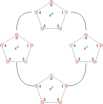
To give a powerful visual intuition of polynomials in quotient rings, consider the following polynomial$1 + 4x + 2x^3 \in \mathbb Z/5\mathbb Z[x] / (x^4+1)$ and its visual representation. For this grade 3 polynomial we have four pentagons, for each coefficient. Each pentagon represents $\mathbb Z/ 5\mathbb Z$. The value of the coefficient is colored with green:

The security of the BGV scheme

Like we said in the introduction, our ciphertexts will be masked with some noise to look as random as possible in order to hide any information an attacker may extract about the message.

In fact it can be proven that the BGV scheme is secure as long as nobody can solve the Ring Learning With Errors (RLWE) problem described below. The parameters of the scheme must be chosen such that there are no known algorithms to solve the underlying RLWE problem in feasable time.

Formally, the idea of "ciphertexts looking like garbage" is called ciphertext indistinguishability. This concept can be formulated using a game between a challenger and an adversary:

• The challenger receives two messages $m_0, m_1$ from the adversary. Then, the challenger encrypts them into $c_0, c_1$.
• Then, the challenger secretly flips a bit $b\in \{0, 1\}$ and sends the ciphertext $c_b$ to the adversary.
• The adversary must guess the bit $b$. After running an efficient algorithm, it outputs a bit $b'$. It wins if $b' = b$.

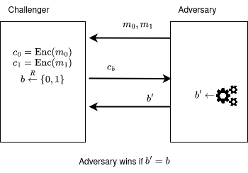
If there exists at least one adversary that can win the game with a probability significantly larger than 1/2 (a coinflip) using a computationally efficient algorithm (something that can run in our universe's lifetime), the challenger's algorithm is considered insecure. When we prove the security of a scheme, we actually show that if an adversary had such an algorithm that can win the security game, he can take that algorithm and use it to solve a problem that is considered computationally hard.

We will now describe the RLWE problem.

Consider the quotient polynomial ring $R_q = \mathbb Z_q[X]/ (X^n + 1)$. This ring has polynomials with degree at most $n$ and integer coefficients in $(-q / 2, q / 2]$.

The RLWE problem - decision
The problem asks to distinguish between the following two distributions:

• $(a_i, b_i)$ with $a_i \xleftarrow R R_q$, $b_i \xleftarrow R R_q$.
• $(a_i, b_i)$ with $a_i \xleftarrow R R_q$, $e_i \leftarrow \chi$, and $b_i = a_i \cdot s + e_i$ for some "small" secret $s \in R_q$ sampled before.

The RLWE problem also has a search version, where given pairs $(a_i, b_i)$, $b_i = a_i \cdot s + e_i$ you need to find $s$. In practice, the decision version is more widely used when proving the security of different schemes.

More details about the RLWE problem can be found in this paper. In essence, by adding some small noise $e_i$, from a Gaussian distribution, we make our secret $s$ unrecoverable even if we have access to many RLWE samples.

The original BGV paper presents the algorithms (encryption, decryption, etc) of a HE scheme based on a more general problem, the General Learning with Errors (GLWE) problem. For simplicity, we work with the RLWE case in this blogpost.

The BGV encryption scheme

Generate the following parameters

• $n$ - degree of $X^n + 1$. $n$ is chosen as a power of 2.
• $q$ - ciphertext modulus.
• $t$ - plainext modulus, $t \ll q$.
• $\chi$ - the noise distribution, a discrete Gaussian.

We consider $R_q = \mathbb Z_q[X] / (X^n + 1)$. This ring has polynomials with degree at most $n$ and integer coefficients in $(-q / 2, q / 2]$.

Note:

• All polynomial operations are considered $\bmod q$ unless otherwise specified, to ease notation.
• When we talk about "small" polynomials, we intuitively think about them having small coefficients.
• Polynomials that come from the noise distribution will be colored with green (ex: $\textcolor{darkgreen}{e}$) and the ones that will come from the secret key distribution will be colored with red (Ex: $\red{s}, \red{u}$).

We will have one secret key $sk$, a public key with two components $pk = (pk_0, pk_1)$, a ciphertext with 2 components $c = (c_0, c_1)$ The messsage will come from the ring $R_t$.

SecretKeyGen(params) -> sk

• Draw $\red{s}$ from a secret key distribution which outputs "small" elements with overwhelming probability. In practice $\red{s} \in \{-1, 0, 1\}^n$, with the probability of sampling $0$ specified as a parameter and the probabilities of sampling $-1$ or $1$ being equal.
• Return the secret key $sk = \red{s}$.

PubKeyGen(sk, params) -> (pk0, pk1)

• Draw a random element $a \xleftarrow R R_q$ and the noise $\textcolor{darkgreen}{e} \leftarrow \chi$.
• Return the public key: $pk = (pk_0, pk_1) = \underbrace{(a \cdot \red{s} + t\textcolor{darkgreen}{e}, -a)}_{\text{RLWE instance-like}}$.

Notice that the public key looks like a RLWE sample, but the error $e$ is multiplied by the plaintext modulus $t$.

Encrypt(m, pk, params) -> (c0, c1)

• Draw the noise $\textcolor{darkgreen}{e_0}, \textcolor{darkgreen}{e_1} \leftarrow \chi$ and a "small" polynomial $\red{u} \in \{-1, 0, 1\}^n$ in the same way as the secret.
• Compute $c_0 = pk_0 \cdot \red{u} + t\textcolor{darkgreen}{e_0} + m$
• Compute $c_1 = pk_1 \cdot \red{u} + t\textcolor{darkgreen}{e_1}$
• Return $c = (c_0, c_1)$.

The ciphertext components $(c_0, c_1)$ are elements in $R_q = \mathbb Z_q[X]/(X^n + 1)$.

Decrypt(c, sk, params)

• Compute $m = c_0 + c_1 \cdot \red{s} \bmod q \bmod t$
• Return $m$.

FHE Operations

Here we will explore the homomorphic properties of the scheme. We refer to the two input message and ciphertext pairs with $(m, c), (m', c')$ and to the resulting message-ciphertext pair with $(m^*, c^*)$.

The goal is to find two functions, $\text{add}, \text{mul}$, that work on ciphertexts, for addition and multiplication, such that:

• when $m^* = m + m'$ we have $c^* = \text{add}(c, c')$ and $\text{Dec}(c^*) = m^*$
• when $m^* = m \cdot m'$ we have $c^* = \text{mul}(c, c')$ and $\text{Dec}(c^*) = m^*$

Recall that $c$ and $c'$ encrypt $m$ and $m'$ i.e.:

FHE Addition

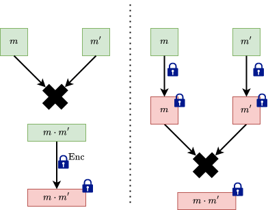
The image on the left performs the addition before the encryption, with the messages in clear. This is not what we want. The image on the right is the desirable outcome, where we encrypt the messages, then perform addition on the encrypted messages.

We define add: add(c, c') -> c*

• $c^*_0 = c_0 + c'_0$
• $c^*_1 = c_1 + c'_1$
• return $c^* = (c^*_0, c^*_1)$

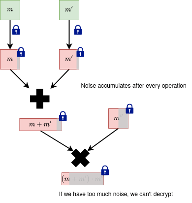
The resulting ciphertext $c^*$ is not fresh anymore (just encrypted), and has a bigger noise than any of the previous ciphertexts that were inputs in the addition operation. In general, using non-fresh ciphertexts $c^*$ to perform future operations will carry over the noise from all the previous operations.

We'll analyse how the noise grows in a dedicated section at the end.

FHE Multiplication

As in the addition case, we want the multiplication to be done on the encrypted messages.

Before describing how we multiply two ciphertexts we need to reinterpret the decryption equation: $c_0 + c_1 \cdot \red{s} \equiv m \bmod t$ as a linear equation: $y = ax + b$ in $\red{s}$.

If we look at adding two such linear equations in $s$ we obtain another linear equation in $\red{s}$: $c_0 + c_1 \cdot \red{s} + c'_0 + c'_1 \cdot \red{s} = \underbrace{(c_0 + c_0')}_{c^*_0} + \underbrace{(c_1 + c'_1)}_{c^*_1} \cdot \red{s}$

However, when multiplying two linear equations in $\red{s}$ we get a quadratic equation ($ax^2 + bx + c$) in $\red{s}$:

We can define mul in the following way: mul(c, c') -> c*

• $c^*_0 = c_0 \cdot c'_0$
• $c^*_1 = c_0 \cdot c'_1 + c_1 \cdot c'_0$
• $c^*_2 = c_1 \cdot c'_1$
• return $c^* = (c^*_0, c^*_1, c^*_2)$

Remarks

• Similarly, as in addition, the noise of the resulting ciphertext $c^*$ increases.
• We increase the number of ciphertext components by 1. This is not sustainable.
• Our decryption equation is linear, however after mul we have a quadratic decryption equation with 3 ciphertexts that doesn't play well with our idea of linear decryption equation.

To solve the remarks the concept of relinearization is introduced.

Relinearization

The concept was explained in the BFV blogpost as well.

Intuition: We want to transform the quadratic equation $c^*_0 + c^*_1 \cdot \red{s} + c^*_2 \cdot \red{s}^2$ in $\red{s}$ into some other linear equation $\hat c_0 + \hat c_1 \cdot \red{\hat s}$ in some other secret key $\red{\hat s}$.

In order to do this we need to give some extra information (a "hint") about the key $\red{s}$ that will help us get $\red{\hat s}$.

Consider the hint to be the pair:

This is very similar to how the public key is generated and we can use the PubKeyGen -> (pk0, pk1) to generate it: $(pk_0 + \red{s}^2, pk_1)$ Intuitively, we use a RLWE sample to hide $\red{s}^2$.

Notice that:

The easiest way to get the term $c^*_2 \red{s}^2$ from the above equation is to multiply it by $c^*_2$. However, $c^*_2$ is a random element in $R_q$ and it will yield some large noise $c^*_2\textcolor{darkgreen}{e}$. So we have to do something smarter.

Key switching v1

Key switching is a variant of relinearization. We start with a ciphertext $c$.

Idea:
Split the ciphertext into multiple "small" ciphertexts (for now think of small as the ciphertext polynomials having small coefficents). We can do this by decomposing the ciphertext coefficients into a small base $T$.

Intuition:
To build an intuition, we can take the most common bases used in representing numbers:

• Base 10: $123_{10} = 3 \cdot 10^0 + 2 \cdot 10 ^1 + 1 \cdot 10^2$
• Base 2: $12_{10} = 1100_2 = 1 \cdot 2^3 + 1 \cdot 2^2 + 0 \cdot 2^1 + 0 \cdot 2^0$

Programmatically, this can be done by dividing the integer by the base $T$ repeatedly and collecting the remainders.

In Python code:

def int2base(x: int, base: int) -> List[int]:
    digits = []
    while x > 0:
        q, r = divmod(x, base)
        digits.append(r)
        x = q
    return digits
    
print(int2base(123, 10))
# [3, 2, 1]
print(int2base(12, 2))
# [0, 0, 1, 1]

A ciphertext component $c \in R_q$ is a polynomial of degree less than $n$, with coefficients in $\{0,1,..,q-1\}$, which we denote as follows: $c(x) = c[0] + c[1]x + ... + c[n-1]x^{n-1}$

We want to write the coefficients $(c[0], ..., c[n-1])$ in base $T$. Since any coefficient is less than $q$, this decomposition has at most $\lfloor \log_T q \rfloor + 1$ terms. For example $c[0] = \sum_{i=0}^{\lfloor \log_T q \rfloor} T^i c[0]^{(i)}$ where $c[0]^{(i)}$ is the corresponding digit $< T$ in the decomposition. Using these digits we can construct the polynomials $c^{(i)}$:

Then using these polynomials we can decompose the original polynomial $c$:

The polynomials $c^{(i)}$ are elements of $R_T$ and for a reasonable small $T$ they have small coefficients ($< T$). For each one of them we generate the hints:

with $a_i \xleftarrow{R} R_q$ and $\textcolor{darkgreen}{e_i} \leftarrow \chi$.

Now we go back to our ciphertext $c^* = (c_0^*, c_1^*, c_2^*)$, the result of EvalMul. We decompose $c^*_2$ in the base $T$ and we get:

Then we construct the new ciphertext $\hat c$ with the two components:

Using the above relations, we obtain the following linear equation:

(the terms containing $a_i \cdot \red{s}$ from $\hat c_0$ and $-a_i \cdot \red{s}$ from $\hat c_1 \cdot \red{s}$ cancel out, $c^*_2$ is reconstructed and we are left with an error term).

Because the relinearization error is a multiple of $t$, it goes away when we decrypt and reduce $\bmod t$ as long as the relinearization error does not wrap $m^* = m\cdot m'$ around $q$.

Remarks

• We need to relinearize after a multiplication.
• A smaller $T$ means we have a smaller noise, but more relinearization keys are needed.
• $T$ is chosen based on what we want to optimize. We usually want to choose $T$ to introduce a noise around the size of the noise in the ciphertexts. Once the noise grows we can use $T^2$ or something else. We can also choose a big $T$ at the start (which introduces lots of starting noise) and we don't need to change it later.

Modulus switching

Task: You want to reduce the noise that accumulates in the ciphertext, after performing homomorphic operations. The modulus switching technique allows us to decrease the noise, to ensure the decryption is still correct after performing homomorphic operations. More analysis is provided in a dedicated section below.

Idea: The technique uses two moduli $Q, q$ with $q < Q$ and $q | Q$. This involves changing the ring where the ciphertexts live, $R_Q$, with a ring $R_q$, that is parametrized by the smaller modulus. When you perform this change, the coefficient ring $\mathbb Z_Q$ is "approximated" by some ring $\mathbb Z_q$, in the intuitive sense that the numbers become smaller (the numbers are scaled down by some factor). As we will see this means that the noise will be smaller in absolute value. Although, the noise will relatively stay the same, since $q < Q$, we mostly care about the magnitude of the noise, especially in multiplications.

You can perform this repeatedly with many moduli $\{q_0, q_1, ..., q_L\}$ with decreasing values to lower the noise after each multiplication.

The easiest way to do this is to scale down the ciphertext's components by $q / Q$ and smartly round in a way to keep the decryption equation correct. To ensure this, we want the scaling to keep the following propriety: $\tilde c_i = c_i \bmod t$ , where $\tilde c_i \approx (q / Q) c_i$ where $i \in \{0, 1\}$.

The two requirements that we want to have are

1. The decryption should be correct (decryption mod $Q$ should be the same as decryption mod $q$): $[c_0 + c_1 \cdot \red{s}]_Q = [\tilde c_0 + \tilde c_1 \cdot \red{s}]_q \bmod t$.
2. The noise scales down.

Rounding
In order for the decryption to be correct we must adjust $c_i$ before scaling by $q / Q$. To do this we add a small correction term $\delta_i$ per component. We require $\delta_i$ to:

1. Only influence the error, hence $\delta_i \equiv 0 \bmod t$ (it will disappear when decrypting)
2. Make the ciphertext to be divisible by $Q / q$:
   $$c_i + \delta_i \equiv 0 \bmod \dfrac Q q \Rightarrow \delta_i \equiv -c_i \bmod \dfrac Q q$$

One easy choice to set the correction terms such that both properties hold is $\delta_i = t [-c_i t^{-1}]_{Q/q}$ where $t^{-1}$ is the inverse of $t$ modulo $Q / q$.

In the end, we define the components $\tilde c_i$ of the modulus switched ciphertext: $\tilde c_i = \dfrac q Q(c_i + \delta_i)$

Key switching v2

Now that we know about modulus switching we introduce a second version to do key switching in BGV. Recall that the key switching technique is used in relinearization, for decreasing the size of the ciphertext obtained in multiplication.

Idea: Given two moduli $q, Q$ with $q < Q$ and $q | Q$, we start with elements in $R_q$ and we make a detour in a ring $R_Q$ with a bigger modulus $Q$ where we perform our relinearization. Then we perform modulus switching to go back to our small ring $R_q$.

We generate the hint:

Recall that $c^* = (c^*_0, c^*_1, c^*_2)$ is the result of the mul. Then we compute the components of the new ciphertext $\hat c$:

Lastly, we scale them both using modulus switching: $\hat c_i = \dfrac q Q (\hat c_i + \delta_i)$ with $\delta_i = t[-c_i t^{-1}]_{Q/q}$, like before.

The relinearization equation looks like this:

Because the relinearization error is a multiple of $t$ (remember that we chose $\delta_i$ to be multiples of $t$ too, to not influence the error), it will go away when we decrypt and reduce $\bmod t$ as long as the relinearization error does not wrap $m^* = m\cdot m'$ around $q$.